accpnt

Time series smoothing using Rust

07/02/2025

I've been self-teaching Rust for a few years now. This language is impressive in terms of its memory handling, albeit sometimes obfuscated by its syntax. However, I trust that it will become a major language in the future. It's been a "learning-by-doing" process for me so far. I’ve immersed myself in hobby projects, initially sparked by techniques related to my master's degree in quantitative analysis.

I started from scratch a small time series smoothing library to gain performance over Python. This open-source project uses the ndarray crate to achieve high-performance manipulation of arrays, inspired by numpy. Luca Palmieri maintains excellent tutorials that helped me get hands-on with ndarray for this purpose.

I initially stumbled upon this physics-based heat equation implementation and decided to implement it in Rust. This port from Python proved to be relatively easy, but I wanted to compare this approach to more standard smoothing techniques, such as the Simple Moving Average (SMA) and Exponential Moving Average (EMA), which are commonly used in finance. This comparison would be useful for benchmarks and empirical evaluations.

The Exponential Moving Average requires a bit of calculus for its implementation, as the adjusted version applies a weighting to previous steps. The Exponentially Weighted Moving Average (EWMA) is a recursive function defined as follows:

smoothing_formula_01a

And the adjusted function that gives more weight to recent observations, while adjusting for bias in small sample sizes, can be expressed as such:

smoothing_formula_01b

I needed to find a quick way to compute EWMA without relying on two for loops, so I included A as a recursive parameter, as shown below:

smoothing_formula_02

This can then be injected into the EWMA equation as follows:

smoothing_formula_03

The associated Rust code is as follows:

let w : f64 = 1.0 - alpha;
y[0] = x[0];

for t in 1..n {
    let atm1 = (1.0 - w.powf((t+1) as f64)) / alpha;
    let at = (1.0 - w.powf(t as f64)) / alpha;
    y[t] = (x[t] + (w * y[t-1] * at)) / atm1;     
}

The heat smoothing technique ultimately turns out to be the slowest method in terms of execution time. But how do these methods compare in terms of modeling? Here's a visual comparison using a historical copper price dataset:

smoothing_comparison

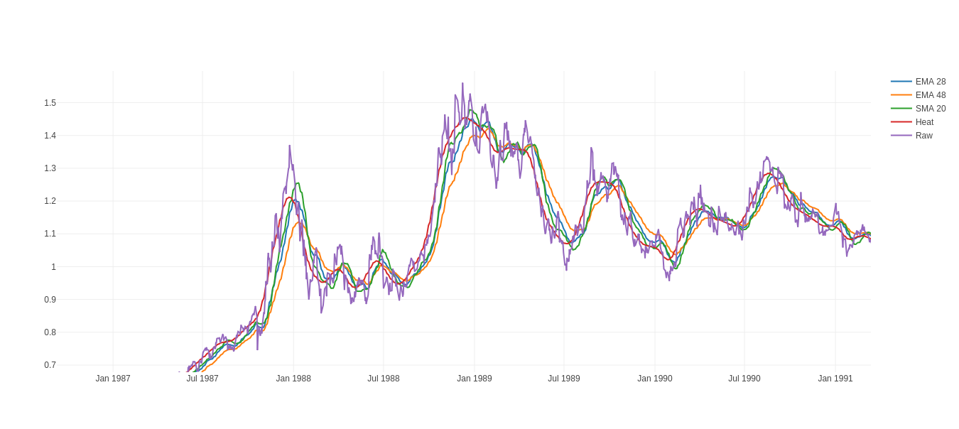
The input parameters make these models hard to compare. But the adjusted EWMA makes it an ideal candidate for performance issue.

Sources are available here. They include unit tests that compare well with the Python implementation.